“Same” materials may have different qualities. For example, their electron mobilities can be different. Classically, the current through a conductor
\[I = n e v S\]Where $n$ is the electron density, $e$ is the electron charge, $v$ is the drift velocity of electrons, $S$ is the cross-sectional area for the electrons to go through. We assumed that electrons are uniformly distributed and all drift at the same speed in an external electric field. The mobility is defined as
\[\mu = v/E\]Where E is the electric field strength. Together we have
\[I = n e (\mu E) S \\ \Rightarrow\\ \mu = I/EneS\\ = I/(U/L)/(neS)\\ = I/U*L/S*1/ne = \sigma/ne\\ \Rightarrow\\ \mu = \sigma/ne=1/n \rho e\]Where $L$ is an arbitrary length along the current, $\sigma$ is the conductivity, $\rho$ is the resistivity.
$e$ is a constant, so $\mu$ is simply the conductivity contributed by a single electron. To measure mobility, one needs to measure electron density and conductivity. It’s not a big problem for 2D and 3D materials, but it might be a problem for 1D materials.
Dimension dependence of the mobility definition
Either $\rho$ or $\sigma$ is dimension dependent. For example, in 3D, the unit of $\rho$ is $\mathrm{\Omega \cdot m}$, in 2D, it is $\mathrm{\Omega}$, while in 1D, it is $\mathrm{\Omega /m}$. Interestingly, the unit of $n$ is also dimension dependent, resulting in a $\mu$ whose unit is independent of the dimension.
Is that just a coincidence? Of cause not. The mobility $\mu$ is defined to be the drift velocity of electrons in the unit electric field. Units of the velocity and the electric field strength do not change in different dimensions.
2D and 3D
We assume materials are uniform. In the 2D cases, the resistivity (conductivity) of an arbitrarily shaped sample can be measured with the Van der Pauw method (hint: an arbitrarily shaped sample with 4 contacts is equal to a half infinity plane with 4 contacts on the edge, with the so-called conformal mapping). Or it can be shaped into a Hall bar and measured with the Hall bar method. Both methods are 4-terminal methods where the resistance due to leads and contacts can be ruled out.
The density can be measured by the famous Hall effect with a magnet, assuming the current density is almost unchanged in the magnetic field. Even though it is strongly altered near the metal contacts because of the Hall angle between the current density and the electrical field which is always perpendicular to the boundary of metal contacts.
3D materials can be made into slabs and be similar to 2D materials. Using the 2D methods we get the sheet resistivity and the sheet density. They can be converted to a 3D version with a known thickness $t$. In fact, we don’t need to know $t$ at all, it cancels with itself when $\rho$ meets $n$. $\rho_{3D} = \rho_s t$, $n_{3D} = n_s/t$ where the subscript $s$ stands for “sheet”. A slab and a real 2D sheet are the same for the mobility measurement!
The mobility calculated with this method is called the Hall mobility because the Hall effect is utilized.
1D
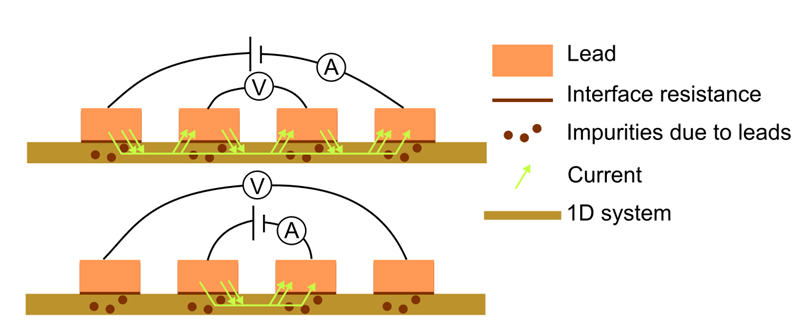
In the 1D case, there is no easy way to measure density and conductivity/resistivity. The Hall effect doesn’t work for 1D. The 4 terminal measurement doesn’t work, neither, because contacts are “invasive” in 1D ([Ref. 1]) in the view of quantum physics. Does it work classically?
As a workaround, people calculate the capacitance, charge the wire with a gate (i.e., change the density), measure the 2 terminal resistance vs the gate voltage. The mobility is then extracted by fitting the curve with known formulas.
Let the capacitance be $C$, the series resistance due to contacts and other stuffs in the 2 terminal measurement is $R_s$, the density is $n = n_0 + C V_g/eL$, where $V_g$ is the gate voltage, $e$ is the elemental charge, $L$ is the length of the junction. The resistivity is $\rho = (R-R_s)/L$, so the mobility is $\mu = 1/n \rho e = 1/(n_0 + C V_g/e L)/((R-R_s)/L)/e$, from which we have
\[R = \frac{L^2}{\mu (n_0 L e + V_g C)} + R_s = \frac{L^2}{\mu C (V_0 + V_g)} + R_s\]or
\[\sigma = \frac{L}{R-R_s} = \mu n_0 e + \frac{\mu C}{L} V_g\]where $V_0 = n_0 L e/C$.
Assume $L$, $C$ are both known constants and $R_s = 0$ (when $R_s « R$), the mobility got by a linear fit is called the field-effect mobility because this method is often used for field-effect transistors (which are usually not 1D…).
Strictly speaking, $L$, $C$, and $R_s$ are not constants against $V_g$. However, we can make them more constant by increasing the length of the junction or rule out the edge effect by measuring junctions with different lengths (can we make identical contacts?). For $C$ it is more tricky because we need to consider not only the edge effect but also the quantum capacitance in series (which is a “bonus” if you want to make your mobility “higher”, but why to bother it?): The Fermi surface moves due to a change of carrier density.
References
- de Picciotto, Rafi, et al. “Four-terminal resistance of a ballistic quantum wire.” Nature 411.6833 (2001): 51-54.