Quantum teleportation

A Single qubit

The bit is a basic unit of information. In classical computers, a bit has binary values, i.e., its state can be either 0 or 1.

The qubit or quantum bit, on the other hand, can be any linear superpositions of states 0 and 1: $|\psi⟩ = \alpha |0⟩ + \beta |1⟩$, where $|\alpha|^2+|\beta|^2 = 1$. Thus a qubit has infinity values (we will see that this can also be true for a classical bit). In quantum physics, the global phase is not important, which means $|\psi⟩$ is equivalent to $e^{i\phi} |\psi⟩$. So we can assume that $\alpha$ is a real number. $\alpha = \cos{\theta/2}$, $\beta = e^{i \phi} \sin{\theta/2}$, $\theta \in [0,\pi]$, $\phi \in [0,2\pi)$, $(1, \theta, \phi)$ is the unit sphere in the spherical coordinate system. This sphere is called the Bloch sphere whose north pole presents state $|0⟩$ and south pole presents state $|1⟩$. In a word, the values of a qubit are as many as points on a sphere (Fun fact: a sphere has one point more than a plane, a plane has the same number of points as a line…).

Multi-value does not make a qubit much different from a classical bit. We can make classical bits more than two values, too. For example, by redefining a “bit” as 10 “binary bits” we get a new “bit” that has 1024 values. Or we can extend the value space of a classical bit just the same way a qubit does: constructing states with a linear combination of 0 and 1. That is not crazy because classical bits are also made based on physical values such as magnetization (hard drive), charge (memory, flash drive), depth of etching (CD), or phase and polarization of electromagnetic wave (WIFI or mobile signal). (Fun fact: in the real world, the bit is redefined so that it is always binary after technique upgrading, such as from 4G to 5G. This is because classical CPUs or algorithms only accept binary bits)

We can conclude that physically both classical bit and qubit have infinity values, only 2 are used in a classical bit while many are used in a qubit.

Two qubits, the magic thing happens

Let’s denote the state of a classical bit by $(\psi)$, a qubit by $|\psi⟩$. When the bit number becomes two, classical bits can be presented by $(\psi_1,\psi_2)$ or $(\psi_1) \otimes (\psi_2)$, the parameter space is simply the tensor product of two single-bit sub-spaces. For two qubits, $|\psi_1,\psi_2⟩$ or $|\psi_1⟩ \otimes |\psi_2⟩$ is merely a subset of all possible states. There are so-called entangled states which can not be presented by the tensor product of two single-bit states. Entangled states are important for quantum computation.

An example of entangled states is $|0,0⟩+|1,1⟩$ (drop the normalization coefficient which is not important). The double-qubit is in the linear combination of states $|0,0⟩$ and $|1,1⟩$. When someone measures one of the two qubits, the result can be either 0 or 1 (this is over-simplified, it can be any points on the Bloch sphere if we carefully design the measurement. Usually, we set up the measurement so that the result is either 0 or 1, i.e. the north and south poles of the Bloch sphere). And the state will be destroyed by that measurement, which is called “collapse”. The magic thing is that the collapsing happens not only in the qubit where the measurement is performed but also in the other qubit. That means $|0,0⟩+|1,1⟩$ becomes either $|0,0⟩$ or $|1,1⟩$ after the measurement, instead of becoming $|0,0⟩+|0,1⟩$ or $|1,0⟩+|1,1⟩$ (why???). Considering the fact that two qubits can be very far away from each other (check this news out, entanglement experiments between a satellite and ground stations), isn’t it crazy that measuring one qubit “changes” the other one immediately while the movement of objects in our university is limited by the speed of the light? Even Einstein didn’t believe it and mocked it as “spooky action at a distance.” However, experiments agree with it.

Some Math

$|0⟩$ and $|1⟩$ are denoted by $[1,0]^T$ and $[0,1]^T$ so that applied mathematics can take over.

(again we drop the normalization coefficient)

Gates can be denoted by matrices or rotations in the Bloch sphere space. For single-bits, there are X, Y, and Z gates which are named after Pauli matrices.

corresponding to rotating 180 degrees around x, y, and z axis. X and Y gates are also the NOT gates because they exchange $|0⟩$ and $|1⟩$.

See Ref. 3 for more gates such as H gate (rotate 180 degrees around (x,y,z) = (1,0,1) direction) or controlled X, controlled Y, controlled Z…

Quantum teleportation

We can create, simulate, visualize quantum circuits with Qiskit, an open-source kit for quantum computers.

The code below is grabbed from Ref. 1.

# Create the circuit for quantum teleportation
# The state in qubit 0 will be copied (teleported) to qubit 2
from qiskit import *
c = QuantumCircuit(3,3)
c.initialize([0.6,0.8], 0)
c.barrier()
c.h(1)
c.cx(1,2)
c.cx(0,1)
c.h(0)
c.barrier()
c.measure([0,1],[0,1])
c.barrier()
c.cx(1,2)
c.cz(0,2)
c.barrier()
c.measure([2],[2])
c.draw()

output:

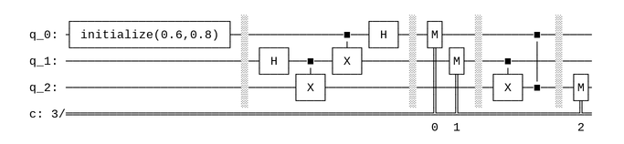
It creates a circuit with 3 qubit and 3 classical bit (for storing measurement results). The state of n-qubit is preseted by $|q_{n-1}q_{n-2}…q_0⟩$, i.e. higher positions first. Same for classical bits and operations. Let’s see what happens in the circuit:

The state is transferred from q0 to q2! We can obtain the result of the quantum circuit with Qiskit, either through a simulator or a real quantum computer shared online by companies such as IBM.

simulator = Aer.get_backend('qasm_simulator')
result = execute(c,backend=simulator,shots=10000).result()
counts = result.get_counts()
print(counts)
print(sum([counts[i] for i in ['000','001','010','011']]))
print(sum([counts[i] for i in ['100','101','110','111']]))

output:

{'000': 904, '001': 941, '010': 927, '011': 844, '100': 1619, '101': 1578, '110': 1640, '111': 1547}
3616
6384

The probability of getting 0 and 1 from qubit 2 is roughly $0.6^2:0.8^2$, as predicted by the theory…

References

1. Programming on Quantum Computers Season 1Ep 5
2. https://medium.com/qiskit/untangling-quantum-teleportation-919cbd673074
3. https://qiskit.org/textbook/ch-states/single-qubit-gates.html