2D (without magnetic fields)
A free electron in a 2D system has the Hamiltonian
\[H_{0} = \frac{1}{2} \frac{p^2}{m}\]The so-called Rashba effect arises when there is a non-zero electric field perpendicular to the 2D plane, which is usually the case for realistic 2D systems due to their lacking mirror symmetry. It is also the simplest approach for spin-orbit coupling because the electric field taken into account for the Rashba effect is uniform [ref_wiki_re].
\[H_{SO} = \frac{1}{2}g \mu_B\frac{1}{m c^2} (\sigma \times p) \cdot E\\ \Rightarrow H_R = \frac{\alpha}{\hbar} (\sigma \times p) \cdot z = \frac{\alpha}{\hbar} (\sigma_x p_y - \sigma_y p_x)\]While the first equation is derivated for a real electron, the second one applys for both electron, and quasi-electron in crystals. In the latter case $\alpha/\hbar$ is not necessary to be $\frac{1}{2} g \mu_B \frac{1}{mc^2} E_0$. [ref_review_rashba]
The total Hamiltonian becomes:
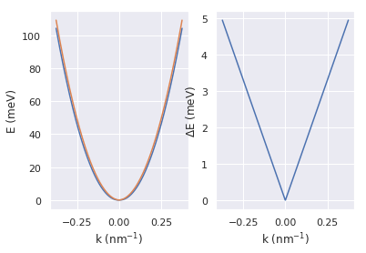
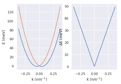
\[H = H_{0} + H_R = \begin{bmatrix} \frac{1}{2} \frac{p^2}{m} & \frac{\alpha}{\hbar} (p_y + i p_x)\\ \frac{\alpha}{\hbar} (p_y - i p_x) & \frac{1}{2} \frac{p^2}{m} \end{bmatrix}\\ \Rightarrow E = \frac{1}{2} \frac{p^2}{m} \pm \frac{\alpha}{\hbar} p = \frac{1}{2} \frac{\hbar^2 k^2}{m} \pm \alpha k\ \text{... [eq_rashba]}\]For more properties, see Fig. 6.3 in Ref. [ref_winkler].
As shown in Equation [eq_rashba], spin-orbit coupling lifts the degeneracy and results in two subbands. These two subbands share the same Fermi energy, so they have different densities, thus two SdH frequencies. A beat pattern may arise in magnetoresistance measurements due to two SdH frequencies(see next section). Let the Fermi energy be $E_F$, with [eq_rashba] we have:
\[k_F = \frac{m}{\hbar^2}(\sqrt{\alpha^2+\frac{2\hbar^2}{m}E_F} \pm \alpha)\]The density of two subbands:
\[n = \frac{1}{(2 \pi)^2}k_F = \frac{n_0}{2} \pm \frac{m}{4\pi^2\hbar^2}\alpha\]Where $n_0$ is the total electron density.
Dresselhaus effect arise when the inversion symmetry is broken by the crystal structure. The general 3D form of Dresselhaus effect is complicated. If we narrow it down to some specific 2D planes, for example, 001 interface in III-V seimiconductors (zincblende structure), we get $H_D = \frac{\beta}{\hbar}(\sigma_x p_x - \sigma_y p_y) + H_D^{higher\ oder}$. For simplicity, let’s temporarily forget about the Dresselhaus effect.
2D (With magnetic fields)
If there is a magnetic field in z direction, say $B = (0,0,B_0)$, another term called Zeeman effect appears:
$H_Z = \frac{1}{2}g \mu_B B\sigma_z$
and $p$ should be replaced with $p-qA$ in previous Hamiltonians. $q = -e$ stands for charge of the particle. $A$ is the Magnetic vector potential. With Landau gauge $A = (0,B_0x,0)$.
\[H_0 = \frac{1}{2m} (p_x^2+(p_y+eB_0x)^2)\\ = \frac{1}{2m} p_x^2+\frac{1}{2} m (\frac{e B_0}{m})^2(x+\frac{p_y}{e B_0})^2\]$H_0$ commutes with $p_y$, we can treat the operator $p_y$ as the number $p_y$. $H_0$ is then equal to the Hamilotnian of a 1D quantum harmonic oscillator located at $x = -\frac{p_y}{eB_0}$ with mass m, angular frequancy $\omega_c = \frac{eB_0}{m}$. So energy levels:
\[E = \hbar \omega_c (n + \frac{1}{2}), n = 1, 2, 3, ...\]For $H_R$, we can still treat $p_y$ as a number,
\[H_R = \frac{\alpha}{\hbar} (\sigma_x (p_y+eB_0x) - \sigma_y p_x)\\ \Rightarrow H_R^2 = (\frac{\alpha}{\hbar})^2((p_y+e B_0 x)^2+p_x^2-\hbar e B_0 \sigma_z)\\ \Rightarrow E^2 = \frac{2 \alpha^2 e B_0}{\hbar} n,\ n = 0, 1, 2, ...\]$E\propto\sqrt{n}$. This is very similar to the Landau level spectrum in graphene [ref_LL_in_graphene].
Please find spectrums of more complicated situations in Ref. [ref_H0+HR], [ref_H0+HR+Hz], [ref_H0+HR+Hd+Hz], you can tell what they are about by these labels. For example, for $H_0+H_R$, Ref. [ref_H0+HR] gives (without a provement):
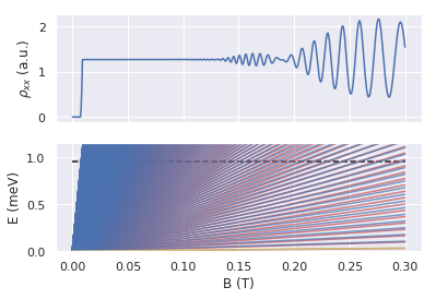
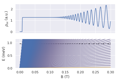
\[E_n = \frac{1}{2} \hbar \omega_c, n=0\] \[E^\pm_n = \hbar \omega_c\left(n\pm\frac{1}{2}\sqrt{1+n\frac{\Delta^2}{E_F\hbar\omega_c}}\right), n=1,2,3,...\]$\Delta = 2\alpha k_F$, is the zero-field spin splitting at $k=k_F$ (see [eq_rashba]). If $E_F»\Delta»\hbar \omega_c$, which is usually guaranteed by the materials and low magnetic fields, for Landau levels near the Fermi surface
\[n \sim \frac{E_F}{\hbar \omega_c}\] \[\Rightarrow n\frac{\Delta^2}{E_F\hbar\omega_c} \sim \frac{E_F}{\hbar \omega_c}\frac{\Delta^2}{E_F\hbar\omega_c} = (\frac{\Delta}{\hbar \omega_c})^2\] \[\Rightarrow E_n^\pm = \hbar \omega_c\left(n\pm\frac{1}{2}\sqrt{1+(\frac{\Delta}{\hbar\omega_c})^2}\right) \sim \hbar\omega_c(n\pm\frac{1}{2}\frac{\Delta}{\hbar\omega_c})\]As there are two sets of Landau levels, each of which has an SdH oscillation with slightly different frequencies, a beat pattern would arise in magnetoresistance measurements. Each time when $\Delta$ is a multiple of $\hbar \omega_c$, the Landau level “ladders” of two subbands coincide with each other near the Fermi energy, the amplitude of SdH oscillation is enhanced, there comes the antinode of the beat pattern. When $\Delta$ is a half-integer multiple of $\hbar \omega_c$, there comes the node of the beat pattern.
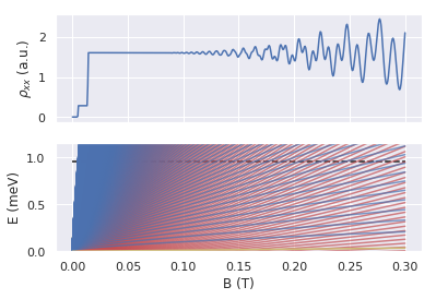
If $\Delta$ is larger,say, $\Delta \sim E_F$,
\[E^\pm_n = \hbar \omega_c\left(n\pm\frac{1}{2}\sqrt{1+n\frac{\Delta^2}{E_F\hbar\omega_c}}\right)\\ \approx \hbar \omega_c\left(n\pm\frac{1}{2}\sqrt{n\frac{\Delta^2}{E_F\hbar\omega_c}}\right)\\ = n \hbar \omega_c \pm\frac{\sqrt{\Delta}}{2}\sqrt{\frac{\Delta}{E_F}}\sqrt{n \hbar \omega_c}\\ = \left(\sqrt{n \hbar \omega_c} \pm\frac{\sqrt{\Delta}}{4}\sqrt{\frac{\Delta}{E_F}}\right)^2-\frac{\Delta}{16}\frac{\Delta}{E_F}\\ \approx \left(\sqrt{n \hbar \omega_c} \pm\frac{\sqrt{\Delta}}{4}\right)^2-\frac{\Delta}{16}\\\]Let $E_F = \Delta= E_n^\pm$, from above equation we get
\[n^-\hbar\omega_c = 1.64E_F\\ n^+\hbar\omega_c = 0.61E_F\]There are still two sets of SdH oscillations. But the frequency difference is too large to make a beat (of course, the density of the two subbands are very different when $\Delta$ is large).
Wires and dots (w/ and w/o magnetic fields)
For an ideal 1D system along x direction ($z=y=0$), assuming $E$ and $B$ are still in z direcion as they were in the 2D case, the total Hamiltonian:
\[H_0+H_R = \frac{p_x^2}{2m}-\frac{\alpha}{\hbar}\sigma_y p_x\]are the same w/ and w/o magnetic fields! And the spectrum is the same as in the case of 2D w/o magnetic fields. Of course (again), the electrons can’t do cyclotron resonance in a 1D world.
But realistic wires are not ideal 1D. They are quasi-1D systems. The y degree of freedom is not frozen, but just quantized. The quantization in y-direction results in many subbands. Assume the confinement potential in y-direction is parabolic, $A = (-yB_0,0,0)$,
\[H_0 = \frac{1}{2m}((p_x-eB_0y)^2+p_y^2)+\frac{m}{2}\omega^2y^2\]There is no $x$ in $H_0$, so $p_x$ commutes with $H_0$, we can take $p_x$ as a number.
\[H_0 = \frac{1}{2m}p_y^2 + (\frac{e^2B_0^2}{2m}+\frac{m\omega^2}{2})y^2 - \frac{eB_0p_x}{m}y+\frac{p_x^2}{2m}=\\ \frac{1}{2m}p_y^2 + \frac{m}{2}(\omega_c^2+\omega^2)y^2 - \omega_c p_x y+\frac{p_x^2}{2m}\xrightarrow{let\ \omega_0=\sqrt{\omega_c^2+\omega^2}}\\ \frac{1}{2m}p_y^2 + \frac{m}{2}\omega_0^2(y-\frac{\omega_c}{\omega_0^2}\frac{p_x}{m})^2 +\frac{p_x^2}{2m}(1-\frac{\omega_c^2}{\omega_0^2})\]Two competing oscillators are combined as one! The degeneracy of Landau levels for 2D is lifted in the quasi-1D situation.
The result for a dot is similar but with two oscillators, as shown in Ref. [ref_dot]:
\[H=\frac{p_1^2+p_2^2}{2m^*}+\frac{m^*}{2}(\omega_1^2q_1^2+\omega_2^2 q_2^2)+\frac{1}{2}g\mu_BB\sigma_z\]The last term is the Zeeman energy. It leads to level crossings at a finite field. At those crossing points, however, spin-orbit coupling lifts the degeneracy and leaves a gap. The anti-crossing gap between the lowest two levels is $2\frac{l}{\lambda_R}E_z$, where $E_z$ is the Zeeman energy, $l=\sqrt{\hbar/m\sqrt{\omega_0^2+\omega_c^2/4}}, \lambda_R=\hbar/m\alpha$. (Ref. [ref_dot]).
import matplotlib.pyplot as plt
import seaborn as sns
sns.set()
import numpy as np
import scipy.constants as sc

def p(alpha,density,m):
  kf = np.sqrt(2*sc.pi*density*1e4)
  x = np.linspace(-kf,kf,500)
  p = np.abs(x)*sc.hbar
  E1 = (p**2/2./m/sc.e-alpha/sc.hbar*p)*1000
  E2 = (p**2/2./m/sc.e+alpha/sc.hbar*p)*1000

  x = x*1e-9
  fig, axes = plt.subplots(1, 2)
  axes[0].plot(x,E1,x,E2)
  axes[0].set_xlabel("k (nm$^{-1}$)");axes[0].set_ylabel("E (meV)")
  axes[1].plot(x,E2-E1)
  axes[1].set_xlabel("k (nm$^{-1}$)");axes[1].set_ylabel("$\Delta$E (meV)")
  plt.show()

alpha = 0.66e-11 #\alpha, in eVm,[ref_H0+HR+Hz]
density = 2.23e12 #cm-2
m = sc.m_e*0.05
p(alpha, density, m)
p(alpha*10, density, m)
def p(delta,density,m,g,Gamma,n1=500,n2=500):
  kf = np.sqrt(2.*sc.pi*density*1e4)
  Ef = sc.hbar**2*kf**2/2./m/sc.e*1000
  B = np.linspace(0,.3,500)#in Tesla
  Ec = B/m*1000.*sc.hbar#cyclotron energy in meV

  n = np.arange(1,n1)
  E1 = np.outer(n,Ec) - 0.5*np.sqrt((1-g*m*0.5)**2*Ec**2+np.outer(n,Ec)*delta**2/Ef)
  sigma1 = np.dot(np.exp(-(Ef-E1)**2/Gamma**2).T,n-0.5)
  n = np.arange(1,n2)
  E2 = np.outer(n,Ec) + 0.5*np.sqrt((1-g*m*0.5)**2*Ec**2+np.outer(n,Ec)*delta**2/Ef)
  sigma2 = np.dot(np.exp(-(Ef-E2)**2/Gamma**2).T,n+0.5)

  fig,axes = plt.subplots(2,1)

  axes[0].plot(B,(sigma1+sigma2)*B**2)
  axes[0].set_ylabel(r"$\rho_{xx}$ (a.u.)")
  axes[0].xaxis.set_ticklabels([])

  axes[1].plot(B,E1.T,color = 'r',alpha=0.7)
  axes[1].plot(B,E2.T,color = 'b',alpha=0.7)
  axes[1].plot(B,Ec*0.5,'y')
  axes[1].hlines(Ef,B[0],B[-1],linestyles='dashed')
  axes[1].set_ylim([0,Ef*1.2])
  axes[1].set_ylabel("E (meV)")
  axes[1].set_xlabel("B (T)");


#  axes[1].set_ylim([3.19,3.2]);


  plt.show()

delta = 0.1 #zero field spin splitting, in meV,[ref_H0+HR+Hz]
density = 2e11 #cm-2
m = sc.m_e*0.5
g = 7#not important
Gamma = 0.02
p(delta,density,m,g,Gamma)
p(delta*0.1,density,m,g,Gamma)
p(delta*10,density,m,g,Gamma)